函数
实数与函数
函数
定义 1.
设为非空数集,若有某种确定的关系(或对应关系),对于每个,都有唯一的一个实数与其对应,则称这个对应关系定义了从到中的函数,记为,或。
称为自变量,称为因变量,称为函数在处的值。
自变量的变化范围称为函数的定义域,记为。
当在定义域中任意变动时,函数值的变化范围称为函数的值域,记为。
函数的运算
-
-
-
-
称为和的复合函数
函数的表示方法
- 显式,
- 隐式,
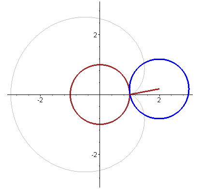
- 参数式,
- 极坐标,
常见函数
- 常值函数:
- 取整函数:
- Dirichlet函数:
- Riemann函数:
阿基米德螺线(Archimedean spiral)
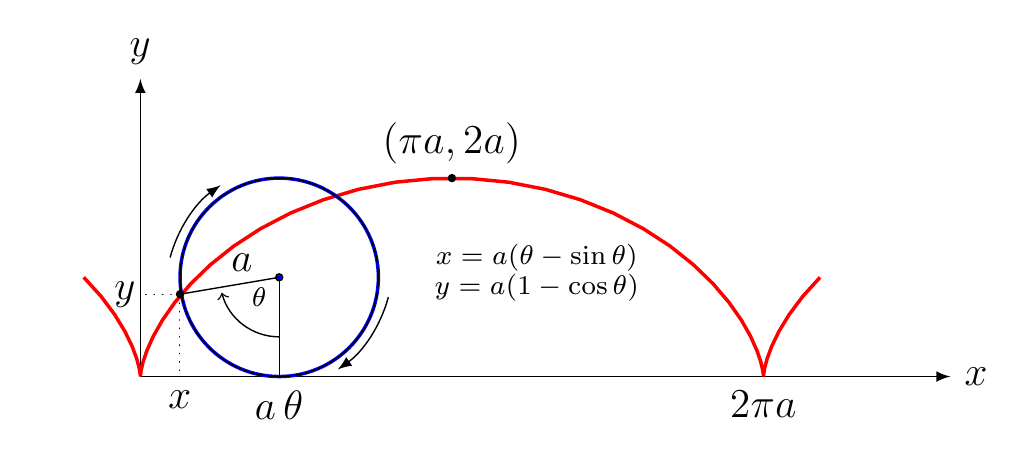
摆线 (cycloid)
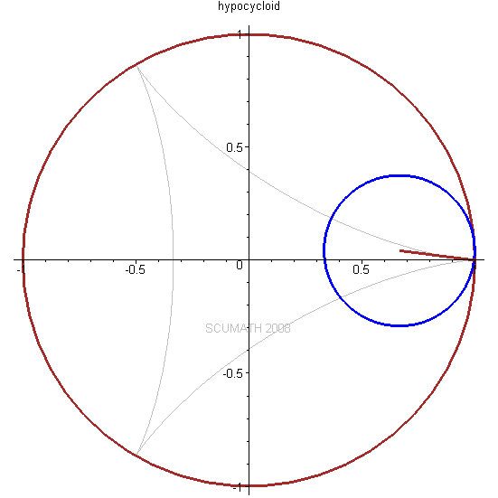
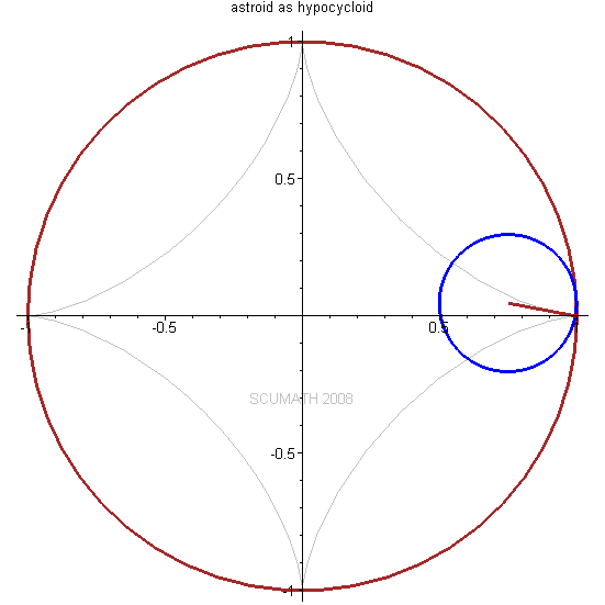
圆内摆线 (Hypocycloid)
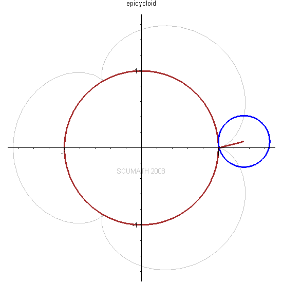
圆外摆线 (epicycloid)
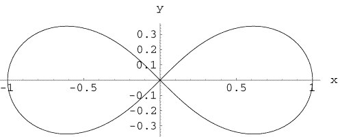
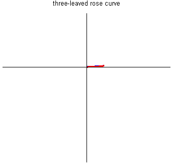
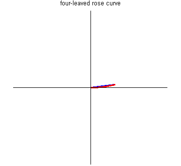
玫瑰线 (Rose Curve)
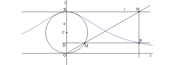
箕舌线 (The Witch of Agnesi)